Exploring Classification in Machine Learning: Algorithms and Use Cases

What is classification?

Classification in machine learning is a method where a machine learning model predicts the label, or class, of input data.

The classification model trains on a dataset, known as training data, where the class (label) of each observation is known, and the model can therefore predict the correct class of unknown observations. The classification model predicts the class/label, based on the features of the training data.

Supervised vs. Unsupervised Learning

Machine learning models are split into three categories depending on whether the dataset has a labeled target variable and the type of label;

Supervised learning

Supervised learning is used on a dataset, known as training data, which must contain a target (dependent) variable that is labeled. The model uses the relationship between the input (independent) and target (dependent) variables in the training data and extrapolates this knowledge to make predictions on a testing dataset.

The model predicts the testing data’s target variable based on the features (independent variables). Regression is used when the target variable is numeric (quantitative) in nature and can be thought of as predicting a value. Classification is used when the target variable is categorical (qualitative) in nature and can be thought of as predicting the class that an unknown observation falls into.

Regression vs Classification

Unsupervised learning

Counter to supervised learning, unsupervised learning uses unlabeled training data. Rather than make predictions, the algorithms provide insight into the hidden patterns within the dataset. Clustering and Dimensionality reduction are examples of unsupervised learning.

Semi-supervised learning

While not a traditional category of machine learning, semi-supervised learning can be used on training data where the target variable contains a mix of both labeled and unlabeled observations.

Semi-supervised classification (induction) is an extension of supervised learning, containing a majority of labeled data, and Constrained clustering (transduction) is an extension of unsupervised learning, containing a majority of unlabeled data.

Reinforcement learning

Reinforcement Learning is a subset of machine learning separate from supervised and unsupervised learning. The software agent is able to interpret its environment and self-trains to make the optimal action through trial and error. It does this through a reward-punishment feedback mechanism which acts as a signal for positive and negative actions, eventually leading it to the optimal solution.

Types of Classification

There are three types of classification based on the nature of the label that is being predicted;

Binary classification

Binary is used when there are two possible outcomes for the label, for example, true/false. Each observation is assigned one and only one label. 

Multi-class classification

Multi-class is used when the dataset has three or more possible classes for the label, for example, red/green/yellow, etc. Each observation is assigned one and only one label.

Multi-label classification

Multi-label is used in a dataset where each observation is assigned a set of multiple labels.

How machine learning models learn

Classification models can learn in two different ways;

Lazy learners

Lazy learners (Instance-based learners) store the training data and delay building a model until it is provided with test data to classify. It predicts the class of a new observation by making local approximations based on the most related stored data. This means that training time is relatively low, however, prediction time is relatively high.

Eager learners

Eager learners are given training data and immediately build a generalized classification model before it receives test data to classify. An eager learner commits to a single hypothesis that covers the entire dataset. This means that training time is relatively high, however, prediction time is relatively low.

Classification Algorithms

There are many different algorithms that all use different approaches to predict classes in machine learning, however, the optimal algorithm depends on the application and dataset that is given.

Naive Bayes

Naive Bayes is an algorithm based on Bayes Theorem that can be used in both binary and multiclass classification. It assumes the features in the dataset are unrelated to each other and contributes to the probability of the class label independently. Naive Bayes is a simple and fast training algorithm that is used for large volumes of data, for example classifying text in the filtering of spam emails.

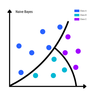
                                                                       Naive Bayes

K-Nearest Neighbors (KNN)

KNN is a lazy learning algorithm and therefore stores all instances of training data points in n-dimensional space (defined by n features). When new testing data is added, it predicts the class of the new observation on a majority vote based on its k nearest neighbors (k number of observations that are closest in proximity).

The newly classified observation then acts as a new training data point for future predictions. KNN is a simple and efficient algorithm that is robust to noisy data, however, can be computationally expensive. An example of KNN in action is recommendation systems used in online shopping.

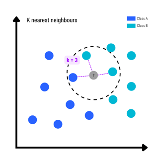
K-Nearest Neighbors (KNN)

Decision Tree (and XGBoost)

The decision tree algorithm builds a top-down tree structure made up of decision nodes (questions about the features) and leaf nodes (class labels), building out the decision nodes until all observations from the training dataset have an assigned class.

The decision tree makes it easy to visualize the classes and requires little data preparation, however, a small adjustment in the training data can completely change the structure of the tree and may make inefficient overly complicated trees when there are many possible classes. This is helped by XGBoosted decision trees.

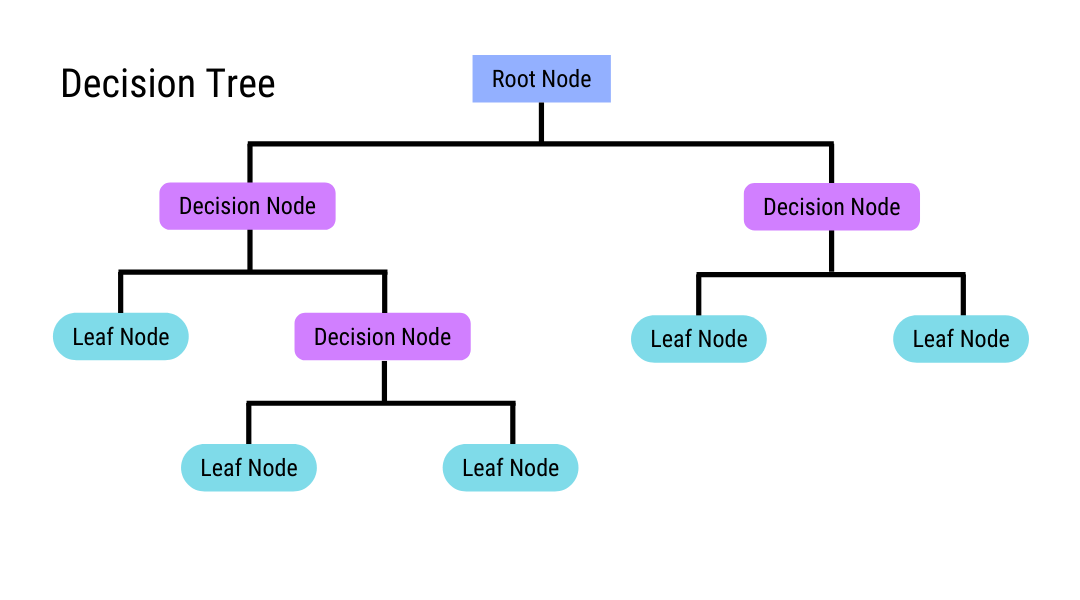
Decision Tree

Random Forest

The Random Forest algorithm constructs multiple decision trees using subsets of the training data and predicts the label of test data by taking the most commonly found (mode) class for observation across the multiple trees. This is done to reduce overfitting that may occur in complex decision trees and is, therefore, more accurate for unseen test data.

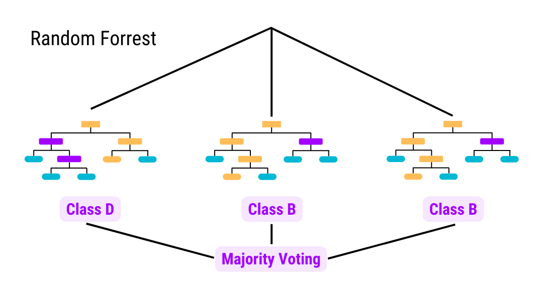
Random Forrest

Support Vector Machine (SVM)

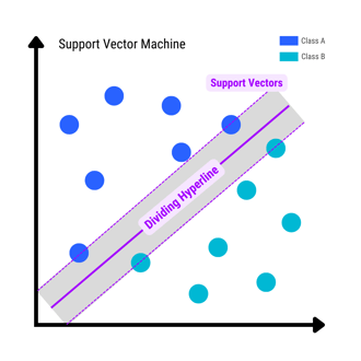
SVM is an eager learning algorithm used for binary classification. Like KNN, SVM places observations in n-dimensional space and separates the two classes using a decision boundary called a hyperplane, which is the widest “gap” (called margin)  between the two. Test observation labels are predicted based on which space they fall into.

SVM works best when there is a clear separation of classes and when there is a large number of features in the training data, however, it is computationally expensive with large data sets and doesn’t perform well when there is noisy data, as there is a smaller separating margin.

Support Vector Machine

 

 

Evaluating Classification Models

Once the classification algorithm has been trained and provided with training data, it is important to check the accuracy of the model through testing, otherwise known as classification evaluation. 

Holdout method

The holdout method is where 80% of the dataset is used for training, and the remaining 20% is used for testing the accuracy of predicted labels. The holdout method is generally used for larger datasets as it is simple and requires less computational power.

Cross-validation

Cross-validation is where the dataset is partitioned into k number of folds (groups). From here, k-1 folds are used for training, and the remaining fold is used for testing, meaning there are k unique train/testing permutations that can be tested. The multiple numbers of tests provide a more accurate representation of how well the model would perform for unseen test data in comparison to the holdout method.

Classification Evaluation Metrics

Classification metrics are the numbers used to measure the effectiveness of the classification model. Before we delve into the measurements, we first need to understand the results which are given in the form of a confusion matrix of size n x n. For a true/false binary classification example, the cells would contain the following:

• True Positive (TP): A positive class that was correctly predicted positive

• True Negative (TN): A negative class that was correctly predicted as negative

• False Positive (FP) [Type 1 error]: A false class that was incorrectly predicted positive

• False Negative (FN) [Type 2 error]: A positive class that was incorrectly predicted negative

Accuracy

Accuracy is the fraction of correctly predicted classifications to total predictions made [(TP+TN) / (TP+TN+FP+FN)]. However accuracy can be misleading when there is an imbalance in the ratio of classes, and in the case of multiclass classification, does not give insight into which classes are being predicted well, which is where the following metrics are helpful.

Recall

Recall is a measurement of how well the classification model predicts the true positive classes and has the equation TP / (TP+FN).

Precision

Precision is a measurement used to understand how well the model performs when it predicts a positive class and has the equation TP/(TP+FP).

Sensitivity

Sensitivity is also known as the true positive rate and is the same as recall.

Specificity

Specificity is also known as the true negative rate and is used to understand how well the classification predicts the true negative classes and has the equation TN/(TN+FP).

F-score

The F-Score combines Recall and Precision into one measurement, however, whereas they both can be used in multiclass classification, the F-Score can only be used in binary classification. It is known as the harmonic mean of Recall and Precision and has the formula TP / (TP+ 0.5*(FP+FN).

Classification Use Cases

As classification is teaching machines to group data into categories by particular criteria, the applications are broad. Some common use cases include:

Detecting Spam Emails

A classification algorithm can be trained to recognize email spam by learning the characteristics of spam vs a non-spam email.

Quality Control

Using production data, a classification model can be trained to detect and classify types of quality control issues like defects.

Fraud Detection

Transaction details data such as amount, merchant, location, time can be used to classify transactions as either legitimate or fraudulent.

Image classification

Machines can analyze pictures through pixel patterns or vectors. Images are high-dimensional vectors, that can be classified into different classes such as a cat, dog, or car. A multi-class classification model can be trained to classify images into different categories.

Document classification

A multi-class classification model can be trained to classify documents into different categories.

There are two types of classification tasks:

Text classification

Concerns defining the type, genre, or theme of the text based on its content.

Visual Classification

Concerns the use of pixels that make up the image to identify the objects pictured, and classify them by behavior or attributes.

Customer Behavior Predictions

Customer buying patterns, website browsing patterns, and other data can be used to classify customer activities into different categories to determine whether a customer is likely to purchase more items, and therefore market to them.

Wrapping up

Hopefully, this blog has given you some insight into classification in machine learning. If you’re looking to start building some classification models for yourself, consider using the AI & Analytics Engine.

Not sure where to start with machine learning? Reach out to us with your business problem, and we’ll get in touch with how the Engine can help you specifically.