In data science, the most popular introductory exercise is the Titanic problem, which is the most popular competition on Kaggle. The task is to use the example Titanic dataset to build a model that predicts whether passengers survive or not.
This problem has been traditionally been done by coding machine learning models, but AutoML platforms like the AI & Analytics Engine has given users the ability to quickly build ML models without coding or extensive data science experience.
In this blog, I'll build a predictive machine learning model using the AI & Analytics Engine. You can follow along by signing up to a free trial of the Engine.
The Engine already contains a Titanic survival prediction app in the playground project that's already loaded into your account. The app contains the data, recipe’s, trained models and predictions for this problem.
Project Homepage
The first thing you’ll need to do is log in to the AI & Analytics Engine. If you haven’t got an account already, you can sign up for a two week free trial for free.
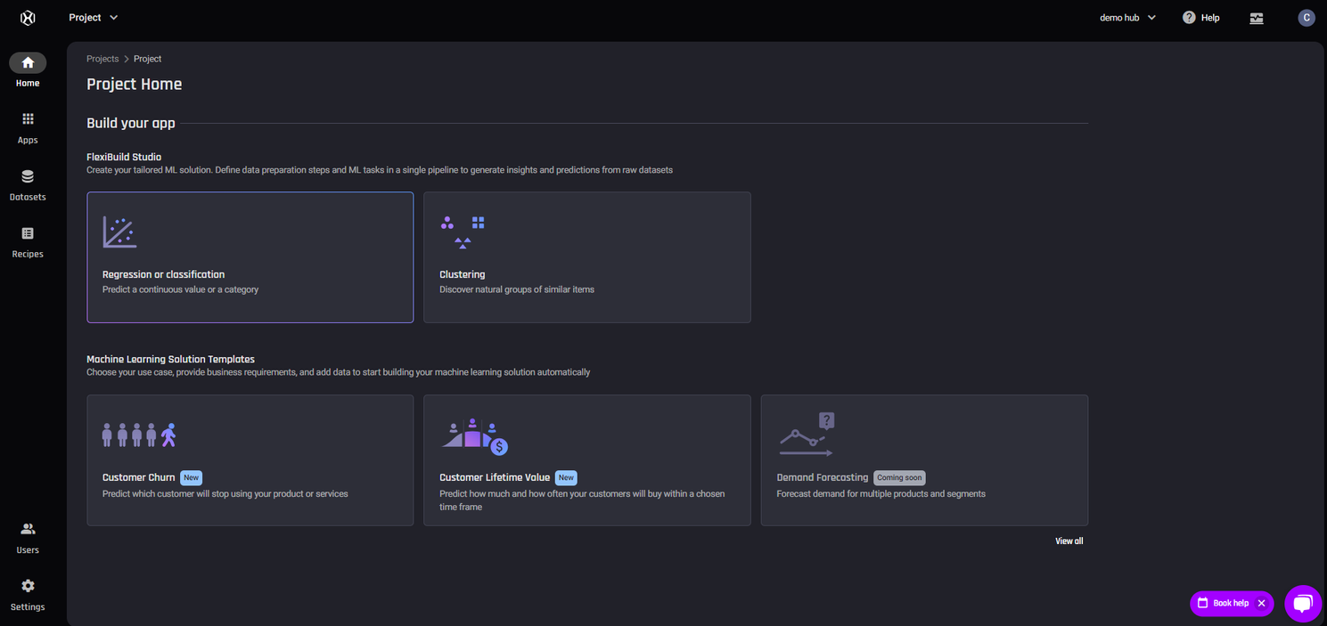
From the project homepage, we’ll want to create a new application, which will house our data, data wrangling recipes, and predictive ML apps.
Select Regression or classification under the FlexiBuild Studio option, as the Titanic exercise is a classification problem.

App builder pipeline
The first section in the App builder pipeline is Prepare data. Upload the train.csv dataset via the local file upload option. The Engine provides a preview of the dataset, and proceed by clicking Create Dataset.
Exploratory data analysis (EDA)
Before we continue in the App builder pipeline, it’s a good idea to get a general understanding of our dataset first. To do this, click view analysis icon next to our uploaded dataset.
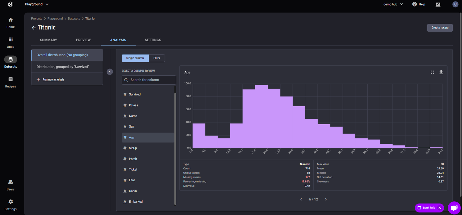
Firstly, we can get a general feel for each column in the dataset by viewing the distribution graph and summary statistics with Single View selected. In the following example of the distribution of age, we notice that most passengers are in their 20s and 30s, but that we’re also missing almost 20% of the data in this column.

Single column analysis of Age
Secondly, we can get a visual representation on how pairs columns correlate with each other by viewing the scatter plots with Pairs selected.
Pairs analysis of Sex, Age and Pclass
Finally, we can see both the Single view and Pairs data when grouped by a specific column by adding a new distribution analysis by selecting Run new analysis. We can use this feature to further understand the data with respect to the target column that we’re interested in, the Survived column.
This gives us some clues as to what features will be impactful in the predictions. The following is Pairs analysis of Sex, Age and Pclass and is grouped by Survived.
The columns are colour coded where pink represents not survived and blue is survived. The top left to bottom right graphs are the Single column visualizations of each feature, and the others are visualizations of pairs of feature.
This analysis gives us clues about what will be important when predicting the Survival column; For example, passengers that are female or in the first/second class have the highest survival rates.
Pairs analysis of Sex, Age and Pclass grouped by Survived
Feature Engineering
It’s possible to use the standard dataset to train our ML models, but to get the highest possible prediction quality possible, we’ll have to do some feature engineering.
Feature engineering involves using the columns, known as features, we have in the dataset to create new features that are highly predictive for the models.
To enter the Engine’s data wrangling feature, click on the uploaded dataset, and select Prepare data.
In the Engine, we have the concept of a recipe. A recipe is a set of data transformation actions, that makes it easy to repeatably apply to new data in a workflows.
I’ve created a recipe of 7 data transformation actions which create three additional features.
Actions 1-2: Create a feature, HasMaidenName, that captures if that person has a maiden name (in parenthesis in the original dataset)
Actions 3-6: Create a feature, NumCabins, that captures how many cabins they have (in a list in the original dataset)
Action 7: Create a feature, FamilySize, that adds that person, and any siblings, spouses, parents and children
This is a creative and experimental step that requires some understanding of the data, so feel free to create your own and see what produces the best results.
Once you’ve done your own data preparation and feature engineering, select the new processed dataset as the training dataset, and click save and continue to resume the app builder pipeline.
The next stage is Defining what to predict. Select survived as the target column. The Engine will recognize that this is a binary classification problem and automatically select that option.
The next stage is Select features, where we must tell the ML models which columns are to be considered when predicting the target column.
The Engine automatically creates a recommended feature set, so we'll use that. We could also experiment with alternative feature sets, that has certain features selected or deselected, later on if we wish.
The final stage is Build Models. We can do this manually, or by selecting the number of models, where we can place restrictions on the training time and expected prediction quality. Let’s train two models with no filters, and click Start Building.
Machine Learning Model Insights
After waiting a short amount of time, our models are trained and ready to go.
On the App Summary Page, we can see that the models have trained on our processed dataset, and are ready to run predictions on our test dataset. But first, let’s navigate to the Models tab and take a look at the Model Leaderboard page.
We trained two models, and the cuML Random Forest Classifier is the most accurate model with 87.88% prediction quality. If we select that model, we can gain some deeper understanding about how the model is performing under the Insights tab.
Performance Insights
The performance insights tab gives us a number of evaluation metrics that we can use to understand how the model performs, including precision, recall and F1 score.
We’re also given a confusion matrix, that describes how the model makes correct and incorrect predictions per class, as well as the ROC curve and Precision-Recall curve.
Feature Importance
The second tab is Feature importance, which describes the degree to which a feature impacts the final prediction of our target variable, in our case, the survival prediction. Here, we can see that our generated features of FamilySize, NumCabins and HasMaidenName all have a relatively low importance.
Our exploratory data analysis gave us an inkling that the sex of the passenger would be an important factor, which is confirmed in our feature importance analysis.
Prediction Explanation
The third tab is Prediction explanation, which uncovers how the particular features affect the prediction result, using real examples from the dataset.
Generating Predictions
Now let’s start generating predictions. On the App Summary Page, click make predictions, and then make one-off prediction.
In the Select model stage, we have to select the model you’d like to generate predictions from. First we’ll choose the cuML Random Forest Classifier as it was our best performing model, but afterwards we’ll also generate predictions from the XGBoost Classifier model as well.
The next stage is Define prediction input, where we have to upload our test dataset. Click choose under data source, and then select import new data source and upload test.csv, and click create dataset. The same data transformation recipe that we created earlier will be applied to this new dataset.
In the Define output columns stage, we have to define the target column’s prediction probability threshold, the probability threshold at which we classify Survived as. Change the output column name to Survived, and we’ll leave the threshold at 0.5 for now, but some experimentation can result in better results depending on the model.
In the next stage, we have the option to export the results to a database or another project in the Engine. If you just want to download the file, you can skip this and click Run prediction.
The progress notification icon will alert you when the prediction is ready. Click on the export icon, and select the As a file option with CSV selected, and then click download.
Prediction Results
The predictions that are downloaded are in the original format of the data, including all features. To submit on Kaggle, you’ll have to ensure the format matches their criteria, which involves removing all columns aside from the PassengerID and Survived column.
Kaggle Results
The results I achieved for each model on the Kaggle competition is as follows:
-
cuML Random Classifier: Score: 0.77033
-
XGBoost Classifier: Score: 0.77272
Some solid results, but there is definitely room for improvement (hint: Feature engineering and prediction probability threshold).
Give it a go for yourself, and let me know if you can beat my results!
